
NSDT工具推荐: Three.js AI纹理开发包 - YOLO合成数据生成器 - GLTF/GLB在线编辑 - 3D模型格式在线转换 - 可编程3D场景编辑器 - REVIT导出3D模型插件 - 3D模型语义搜索引擎 - Three.js虚拟轴心开发包 - 3D模型在线减面 - STL模型在线切割
有许多 python 包与 Dask 紧密集成,可以实现并行数据处理。例如,考虑 xarray 包。该包用于读取 netcdf、hdf5、zarr 文件格式的数据集。当从多个文件读取数据时,Dask 就会发挥作用,其中每个文件都被视为一个块,或者通过显式指定 chunks 参数来描述如何对数据进行分块。
laspy python 包用于读取 3D 点云数据,但不幸的是它缺乏与 Dask 的集成,但当从多个文件读取数据时仍然可以使用它。尽管这种从多个文件加载数据的技术众所周知,但块参数功能增加了很大的灵活性。在本文中,演示了此类功能。
可以在我们的 Gitlab 存储库中找到本文的更永久版本(包含更新和修复)。
1、3D 点云格式 – Las/Laz
本部分为las 格式的简要概述。
3D 点云数据存储为 las 文件。如下图所示,las文件由头、变长记录、点云记录和扩展变长记录组成。根据 las 格式规范的版本,点云记录中存储的字段的细节可能会有所不同,并且可能没有扩展的可变长度记录。
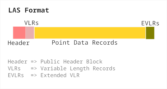
标头部分包含有关文件内容的元数据,例如格式版本、点云记录数量、每个记录的大小(以字节为单位)、点云记录开始的偏移字节、记录中字段的数据类型、最小和最大值空间坐标、比例因子等,
laspy 包提供的便利功能不仅可以读取点云记录,还可以调查元数据。也许从元数据中找出的一件有趣的事情是加载 las 文件的内存要求。这是一个名为 info 的小实用函数来提供此信息。
import humanize
import laspy
import os

def info(filename):
    naturalsize = lambda x: humanize.naturalsize(x, binary=True)
    with open(filename, "rb") as fid:
        reader = laspy.LasReader(fid)
        npoints = reader.header.point_count
        point_size = reader.header.point_format.size
        memory_size = npoints * point_size
    print(f"Filesize on disk: {naturalsize(os.path.getsize(filename))}")
    print(f"Is data compressed: {reader.header.are_points_compressed}")
    print(f"records (points): {npoints} ({humanize.intword(npoints)})")
    print(f"Each record size: {point_size} ({naturalsize(point_size)})")
    print(f"Memory required: {memory_size} ({naturalsize(memory_size)})")
使用info函数确定名为densel-20230906-103153.laz的las文件的内存要求:
filename = "./dense1-20230906-103153.laz"
info(filename)
结果如下:
Filesize on disk: 2.1 GiB
Is data compressed: True
records (points): 148919876 (148.9 million)
Each record size: 54 (54 Bytes)
Memory required: 8041673304 (7.5 GiB)
虽然该文件在磁盘中仅占用 2.1 GiB,但内存中未压缩的数据至少需要 4 倍的内存空间(7.5 GiB)。该功能对于规划计算节点资源需求非常有用。 “每个记录大小”表示在磁盘上存储压缩数据所需的字节数。
2、分块读取Las文件
正如简介中提到的,其想法不是将文件物理分割成多个较小的文件,而是在逻辑上将单个文件分割成多个块,以便 Dask 可以处理这些块。出现的直接问题是如何对数据进行分块。标准可以是以下任意一项:
- 按每个块的点数(例如:每个块 200 万个)
- 按每个块的大小(例如:每个块 100MB)
- 将数据划分为 n 个分区(例如:100 个分区,即 100 个块)
扩展info函数以合并这些功能:
import re
from dask.utils import byte_sizes


def convert_humansize_to_bytes(value: str):
    match = re.search('([^\.eE\d]+)', str(value))
    nbytes = 1
    if match:
        start = match.start()
        text = match.group().strip().lower()
        nbytes = byte_sizes[text]
        value = value[:start]
    value = int(float(value)) * nbytes
    return value


def info(
        filename,
        partition_by_size: str = None,
        partition_by_points: int = None,
        partition_by_partitions: int = None,
        echo: bool = True,
        return_batch_points: bool = False
):

    naturalsize = lambda x: humanize.naturalsize(x, binary=True)
    with open(filename, "rb") as fid:
        reader = laspy.LasReader(fid)
        npoints = reader.header.point_count
        point_size = reader.header.point_format.size
        memory_size = npoints * point_size
        if echo:
            print(f"Filesize on disk: {naturalsize(os.path.getsize(filename))}")
            print(f"Is data compressed: {reader.header.are_points_compressed}")
            print(f"records (points): {npoints} ({humanize.intword(npoints)})")
            print(f"Each record size: {point_size} ({naturalsize(point_size)})")
            print(f"Memory required: {memory_size} ({naturalsize(memory_size)})")
    if partition_by_partitions:
        batch_size = round(memory_size/partition_by_partitions/10)*10
        batch_points = round(batch_size/point_size/10)*10
        batch_size = batch_points * point_size
    elif partition_by_points:
        batch_points = partition_by_points
        batch_size = batch_points * point_size
    elif partition_by_size:
        batch_size = convert_humansize_to_bytes(partition_by_size)
        batch_points = round(batch_size/point_size/10)*10
        batch_size = batch_points * point_size
    else:
        batch_size = memory_size
        batch_points = npoints

    nbatches = len(range(0, npoints, batch_points))
    if any([partition_by_partitions, partition_by_points, partition_by_size]) and echo:
        print("---")
        print(f"  chunk_size = {batch_size} ({naturalsize(batch_size)})")
        print(f"  points_per_chunk = {batch_points} ({humanize.intword(batch_points)})")
        print(f"  nchunks = {nbatches}")
        print("---")
    if return_batch_points:
        return batch_points
尝试使用info功能来查看这些不同选项的实际效果。
按大小分块,将数据分块,每个块大约为 100 MB
>>> filename = "./dense1-20230906-103153.laz"
>>> info(filename, partition_by_size="100MB")
结果如下:
Filesize on disk: 2.1 GiB
Is data compressed: True
records (points): 148919876 (148.9 million)
Each record size: 54 (54 Bytes)
Memory required: 8041673304 (7.5 GiB)
---
  chunk_size = 99999900 (95.4 MiB)
  points_per_chunk = 1851850 (1.9 million)
  nchunks = 81
---
你可能会注意到,块大小略小于 100 MB。这是因为 1MB 转换为 1000 字节。如果每 MB 需要 1024 字节,则使用 MiB 表示法:
>>> info(filename, partition_by_size="100MiB")结果如下:
Filesize on disk: 2.1 GiB
Is data compressed: True
records (points): 148919876 (148.9 million)
Each record size: 54 (54 Bytes)
Memory required: 8041673304 (7.5 GiB)
---
  chunk_size = 104857740 (100.0 MiB)
  points_per_chunk = 1941810 (1.9 million)
  nchunks = 77
---
按点分块:
>>> info(filename, partition_by_points=10_00_000)结果如下:
Filesize on disk: 2.1 GiB
Is data compressed: True
records (points): 148919876 (148.9 million)
Each record size: 54 (54 Bytes)
Memory required: 8041673304 (7.5 GiB)
---
  chunk_size = 54000000 (51.5 MiB)
  points_per_chunk = 1000000 (1.0 million)
  nchunks = 149
---
按分区分块:
>>> info(filename, partition_by_partitions=100)结果如下:
Filesize on disk: 2.1 GiB
Is data compressed: True
records (points): 148919876 (148.9 million)
Each record size: 54 (54 Bytes)
Memory required: 8041673304 (7.5 GiB)
---
  chunk_size = 80416800 (76.7 MiB)
  points_per_chunk = 1489200 (1.5 million)
  nchunks = 100
---
info 函数显示了如何将文件逻辑划分为多个块,下一步是创建一个实际将文件划分为块的函数。
3、分割Las文件
下面的 dask_reader 函数将文件分成块并根据需要延迟加载它们:
import dask
import dask.dataframe as dd
import pandas as pd
import numpy as np


@dask.delayed
def _dask_offset_reader(filename, offset, npoints, scaled=False, func=lambda x:x):
    with open(filename, "rb") as fid:
        reader = laspy.LasReader(fid)
        reader.seek(offset)
        pts = reader.read_points(npoints)
        if scaled:
            xyz_scaled = {'x': pts.x.scaled_array(),
                          'y': pts.y.scaled_array(),
                          'z': pts.z.scaled_array()}
        data = pts.array
    d = pd.DataFrame(data)
    d.index = np.arange(offset, offset+npoints)
    if scaled:
        d['x'] = xyz_scaled['x']
        d['y'] = xyz_scaled['y']
        d['z'] = xyz_scaled['z']
    d = func(d)
    return d


def dask_reader(
        filename,
        partition_by_size=None,
        partition_by_points=None,
        partition_by_partitions=None,
        scaled=False,
        func=lambda x:x,
):
    batch_points = info(
        filename,
        partition_by_size,
        partition_by_points,
        partition_by_partitions,
        echo=False,
        return_batch_points=True)

    with open(filename, "rb") as fid:
        reader = laspy.LasReader(fid)
        dtype = reader.header.point_format.dtype()
        #meta = pd.DataFrame(np.empty(0, dtype=dtype))
        npoints = reader.header.point_count
        pairs = [(batch_points, offset)
                 for offset in range(0, npoints, batch_points)]
        batch_pts, offset = pairs.pop(-1)
        batch_pts = npoints - offset
        pairs.append((batch_pts, offset))

    lazy_load = []
    for points, offset in pairs:
        lazy_func = _dask_offset_reader(filename, offset, points, scaled=scaled, func=func)
        lazy_load.append(lazy_func)
    meta_dtype = _dask_offset_reader(filename, 1, 1, scaled=scaled, func=func).compute().to_records().dtype
    meta = pd.DataFrame(np.empty(0, dtype=meta_dtype))
    return dd.from_delayed(lazy_load, meta=meta)
以下是有关如何设置 dask 来加载此数据的工作流程。
设置 dask 集群和客户端:
>>> from dask.distributed import Client, LocalCluster
>>> cluster = LocalCluster(n_workers=12, threads_per_worker=2)
>>> client = Client(cluster)
>>> print(client)
<Client: 'tcp://127.0.0.1:33430' processes=12 threads=24, memory=376.31 GiB>
读取数据:
>>> df = dask_reader(filename, partition_by_size='200MiB')
>>> print(df.head())
            X       Y       Z  intensity  bit_fields  classification_flags  \
    0  237355  566872  368473         13          17                     0
    1  258448  570271  368929          0          33                     0
    2  236036  565853  365470         19          34                     0
    3  270386  571869  368003         44          17                     0
    4  267408  570521  364769         17          33                     0

       classification  user_data  scan_angle  point_source_id    gps_time  \
    0               0          0           0                0  290384.293
    1               0          0           0                0  290384.293
    2               0          0           0                0  290384.293
    3               0          0           0                0  290384.293
    4               0          0           0                0  290384.293

       echo_width  fullwaveIndex  hitObjectId  heliosAmplitude
    0         0.0        2829327        21450       201.914284
    1         0.0        2829328        21450         7.727883
    2         0.0        2829328        21450       292.342904
    3         0.0        2829329        21450       684.970443
    4         0.0        2829330        21450       271.545107
那么,问题是,使用 dask 在速度方面有什么好处吗?计时操作:dask 与非 dask
%%time
hitobjectids = df['hitObjectId'].unique().compute()


CPU times: user 642 ms, sys: 324 ms, total: 966 ms
Wall time: 8.52 s


%%time
data = laspy.read(filename)
h = np.unique(data['hitObjectId'])


CPU times: user 2min 10s, sys: 4.06 s, total: 2min 14s
Wall time: 13.6 s
嗯,使用 Dask 性能会好一点,但并不显着。这里发生了两件事,从磁盘加载数据(I/O 操作)以及随后的一些分析操作。考虑单独测量分析部分的时序,而不是测量这些操作组合的时序。
使用 Dask 将数据加载到内存中:
%%time
df = df.persist()
结果如下:
CPU times: user 12.5 ms, sys: 7.97 ms, total: 20.5 ms
Wall time: 19.1 ms
由于持久化是非阻塞操作,因此数据加载部分发生在后台。 dask 工作人员需要几秒钟的时间才能将数据加载到内存中。
等待几秒钟后,重新运行分析部分。
%%time
hitobjectids = df['hitObjectId'].unique().compute()


CPU times: user 47.1 ms, sys: 27.8 ms, total: 74.9 ms
Wall time: 105 ms
在没有 dask 的情况下重新运行分析部分:
%%time
h = np.unique(data['hitObjectId'])

CPU times: user 4.6 s, sys: 677 ms, total: 5.28 s
Wall time: 4.87 s
现在,这是性能上的显着差异。 Dask 工作流程完全优于通常的工作流程。
4、结束语
在这个特定示例中,源文件需要大约 9GB 内存来加载整个数据集,该数据集可以轻松放入单个节点内存中。对于不适合单个节点的较大数据集, dask_jobqueue 包可以进行分布式计算。在这种情况下,只有集群设置部分不同,其余工作流程保持不变。
本文的目的是展示使用块功能的 3D 点云数据的 Dask 工作流程。如图所示,只需很少的辅助函数,就可以使用 dask 直接读取 3D 点云数据。即使这里显示的分析部分非常有限,使用 dask 的性能优势也很明显。
dask_reader 接受可选的缩放参数,用于缩放 x、y、z 值。可选的 func 参数旨在操作 pandas 数据帧。例如,仅返回选定的列。提供一个接收数据帧作为输入的自定义函数,并且返回值必须是数据帧。
原文链接:Parallel 3D Point Cloud Data analysis with Dask
BimAnt翻译整理,转载请标明出处


