
NSDT工具推荐: Three.js AI纹理开发包 - YOLO合成数据生成器 - GLTF/GLB在线编辑 - 3D模型格式在线转换 - 可编程3D场景编辑器 - REVIT导出3D模型插件 - 3D模型语义搜索引擎 - AI模型在线查看 - Three.js虚拟轴心开发包 - 3D模型在线减面 - STL模型在线切割 - 3D道路快速建模
神经辐射场或 NeRF 是深度学习和计算机视觉领域中一个相当新的范例。 在 ECCV 2020 论文“NeRF: Representing Scenes as Neural Radiance Fields for View Synthesis”(获得最佳论文荣誉奖)中,该技术迅速流行起来,迄今为止已获得近 800 次引用[1]。 该方法标志着机器学习处理 3D 数据的传统方式发生了巨大变化。 视觉效果当然也有那种“哇”的因素,你可以在项目页面和他们的原始视频(下面)中看到。

在本教程中,我们将介绍 NeRF 的基本组件以及如何将它们组合在一起以训练我们自己的 NeRF 模型。 然而,在我们开始之前,让我们先来看看 NeRF 到底是什么,以及是什么让它如此具有突破性。本文代码可以查阅 Google Colab notebook 。
1、什么是 NeRF?
简而言之,NeRF 是一种生成模型,以图像集合和准确姿势(例如位置和旋转)为条件,允许生成图像共享的 3D 场景的新视图,这个过程通常称为“新视图合成。”不仅如此,NeRF还将场景的 3D 形状和外观明确定义为连续函数,你可以使用它来执行诸如通过Marching Cubes生成 3D 网格等操作。
关于 NeRF,有一件事你可能会感到惊讶:尽管它们直接从图像数据中学习,但它们既不使用卷积层也不使用变换器层(至少在原始论文中是这样)。 NeRF 的一个低估的好处是压缩;在 5-10MB 时,NeRF 模型的权重可能小于用于训练它们的图像集合。
多年来,为机器学习应用程序表示 3D 数据的正确方法一直是争论的主题。许多技术已经出现,从 3D 体素到点云再到带符号的距离函数(有关一些常见 3D 表示的更多详细信息,请参阅我的 MeshCNN 文章)。他们最大的共同缺点是初始假设:大多数表示都需要 3D 模型,要求你使用摄影测量(非常耗时和数据)和 LiDAR(通常昂贵且难以使用)等工具生成 3D 数据或者付钱请艺术家为你制作 3D 模型。此外,许多类型的物体,例如高反射物体、“网状”物体(例如灌木和铁丝网围栏)或透明物体,都无法按比例扫描。 3D 重建方法通常也存在重建误差,这会导致影响模型精度的阶梯效应或漂移。
相比之下,NeRF 依赖于一个古老而优雅的概念,称为 或辐射场。光场是描述光在整个 3D 体积中如何传输的函数。它描述了光线穿过空间中每个 x=(x, y, z) 坐标并沿每个方向 d 移动的方向,描述为 θ 和 φ 角或单位向量。它们共同形成一个 5D 特征空间,用于描述 3D 场景中的光传输。 NeRF 受此表示的启发,尝试近似从该空间映射到由颜色 c=(R,G,B) 和密度 σ 组成的 4D 空间的函数,你可以将其视为光的可能性在此 5D 坐标空间中的射线被终止(例如通过遮挡)。因此,标准 NeRF 是 F 形式的函数:(x,d) -> (c,σ)。
原始 NeRF 论文使用直接在一组具有已知姿势的图像上训练的多层感知器对该函数进行参数化(可以通过任何运动结构应用程序获得,例如 COLMAP、Agisoft Metashape、Reality Capture 或 Meshroom)。这是称为广义场景重建的一类技术中的一种方法,旨在直接从图像集合中描述 3D 场景。这种方法为我们提供了一些非常好的属性:
- 直接从数据中学习
- 场景的连续表示允许非常薄和复杂的结构,例如树叶或网格
- 隐式说明物理特性,如镜面反射和粗糙度
- 隐式表示场景中的照明
从那以后,一连串的论文试图通过少镜头和单镜头学习[2, 3],支持动态场景[4, 5],将光场概括为特征场等特征来扩展原始功能[ 6],从来自网络的未校准图像集合中学习[7],结合 LiDAR 数据[8],大规模场景表示[9],没有神经网络的学习[10],等等。有关 NeRF 研究的一些重要概述,请参阅 Frank Dellaert 撰写的 2020 年的这篇重要概述和 2021 年的另一篇概述。
2、NeRF架构
仅使用此功能,如何生成新颖的图像仍然不是很明显。总的来说,给定一个训练有素的 NeRF 模型和一个具有已知姿势和图像尺寸的相机,我们通过以下过程构建场景:
- 对于每个像素,通过场景行进相机光线以在 (x, d) 位置收集一组样本。
- 使用每个样本的 (x, d) 点和观察方向作为输入以产生输出 (c,σ) 值(本质上是 rgbσ)。
- 使用经典的体绘制技术构建图像。
辐射场函数只是几个组件之一,一旦组合在一起,就可以创建之前看到的视频中看到的视觉效果。还有几个组件,我将在本教程中访问每个组件。总体而言,我们将涵盖以下组件:
- 位置编码
- 辐射场函数逼近器(在本例中为 MLP)
- 可微分体积渲染器
- 分层抽样
- 分层体积抽样
我写这篇文章的目的是尽可能清晰,所以我将每个组件的关键元素提取到尽可能简洁的代码中。我使用了 GitHub 用户 bmild 的原始实现和 GitHub 用户 yenchenlin 和 krrish94 的 PyTorch 实现作为参考。
3、位置编码器
与 2017 年推出的极其流行的Transformer模型非常相似[11],NeRF 也受益于位置编码器作为其输入,尽管原因不同。 简而言之,它使用高频函数将其连续输入映射到更高维空间,以帮助模型学习数据中的高频变化,从而产生更清晰的模型。 这种方法避免了神经网络对低频函数的偏见,允许 NeRF 表示更清晰的细节。 作者参考了 ICML 2019 上的一篇论文,以进一步阅读这一现象 [12]。
如果你熟悉位置编码器,NeRF 实现是相当标准的。 它具有与原版标志相同的交替正弦和余弦表达式。
class PositionalEncoder(nn.Module):
  r"""
  Sine-cosine positional encoder for input points.
  """
  def __init__(
    self,
    d_input: int,
    n_freqs: int,
    log_space: bool = False
  ):
    super().__init__()
    self.d_input = d_input
    self.n_freqs = n_freqs
    self.log_space = log_space
    self.d_output = d_input * (1 + 2 * self.n_freqs)
    self.embed_fns = [lambda x: x]

    # Define frequencies in either linear or log scale
    if self.log_space:
      freq_bands = 2.**torch.linspace(0., self.n_freqs - 1, self.n_freqs)
    else:
      freq_bands = torch.linspace(2.**0., 2.**(self.n_freqs - 1), self.n_freqs)

    # Alternate sin and cos
    for freq in freq_bands:
      self.embed_fns.append(lambda x, freq=freq: torch.sin(x * freq))
      self.embed_fns.append(lambda x, freq=freq: torch.cos(x * freq))

  def forward(
    self,
    x
  ) -> torch.Tensor:
    r"""
    Apply positional encoding to input.
    """
    return torch.concat([fn(x) for fn in self.embed_fns], dim=-1)
4、辐射场函数
在原始论文中,辐射场函数由 NeRF 模型表示,这是一个相当典型的多层感知器,它将编码的 3D 点和视图方向作为输入,并返回 RGBA 值作为输出。 虽然本文使用神经网络,但此处可以使用任何函数逼近器。 例如,Yu 等人的后续论文。 称为 Plenoxels 的方法使用球谐函数基来代替训练速度提高几个数量级,同时获得有竞争力的结果 [10]。
NeRF 模型有 8 层深,大多数层的特征维度为 256。 残差连接位于第 4 层。在这些层之后,生成 RGB 和 σ 值。 RGB 值用线性层进一步处理,然后与视图方向连接,然后通过另一个线性层,最后在输出端与 σ 重新组合。
class NeRF(nn.Module):
  r"""
  Neural radiance fields module.
  """
  def __init__(
    self,
    d_input: int = 3,
    n_layers: int = 8,
    d_filter: int = 256,
    skip: Tuple[int] = (4,),
    d_viewdirs: Optional[int] = None
  ):
    super().__init__()
    self.d_input = d_input
    self.skip = skip
    self.act = nn.functional.relu
    self.d_viewdirs = d_viewdirs

    # Create model layers
    self.layers = nn.ModuleList(
      [nn.Linear(self.d_input, d_filter)] +
      [nn.Linear(d_filter + self.d_input, d_filter) if i in skip \
       else nn.Linear(d_filter, d_filter) for i in range(n_layers - 1)]
    )

    # Bottleneck layers
    if self.d_viewdirs is not None:
      # If using viewdirs, split alpha and RGB
      self.alpha_out = nn.Linear(d_filter, 1)
      self.rgb_filters = nn.Linear(d_filter, d_filter)
      self.branch = nn.Linear(d_filter + self.d_viewdirs, d_filter // 2)
      self.output = nn.Linear(d_filter // 2, 3)
    else:
      # If no viewdirs, use simpler output
      self.output = nn.Linear(d_filter, 4)

  def forward(
    self,
    x: torch.Tensor,
    viewdirs: Optional[torch.Tensor] = None
  ) -> torch.Tensor:
    r"""
    Forward pass with optional view direction.
    """

    # Cannot use viewdirs if instantiated with d_viewdirs = None
    if self.d_viewdirs is None and viewdirs is not None:
      raise ValueError('Cannot input x_direction if d_viewdirs was not given.')

    # Apply forward pass up to bottleneck
    x_input = x
    for i, layer in enumerate(self.layers):
      x = self.act(layer(x))
      if i in self.skip:
        x = torch.cat([x, x_input], dim=-1)

    # Apply bottleneck
    if self.d_viewdirs is not None:
      # Split alpha from network output
      alpha = self.alpha_out(x)

      # Pass through bottleneck to get RGB
      x = self.rgb_filters(x)
      x = torch.concat([x, viewdirs], dim=-1)
      x = self.act(self.branch(x))
      x = self.output(x)

      # Concatenate alphas to output
      x = torch.concat([x, alpha], dim=-1)
    else:
      # Simple output
      x = self.output(x)
    return x
5、可微体积渲染器
RGBA 输出点位于 3D 空间中,因此要将它们合成到图像中,我们需要应用本文第 4 节的方程式 1-3 中描述的体积积分。 本质上,我们对每个像素的射线沿线的所有样本进行加权和,以获得该像素的估计颜色值。 每个 RGB 样本都由其 alpha 值加权。 更高的 alpha 值表示采样区域不透明的可能性更高,因此沿着光线更远的点更有可能被遮挡。 累积乘积确保那些进一步的点被抑制。
def raw2outputs(
  raw: torch.Tensor,
  z_vals: torch.Tensor,
  rays_d: torch.Tensor,
  raw_noise_std: float = 0.0,
  white_bkgd: bool = False
) -> Tuple[torch.Tensor, torch.Tensor, torch.Tensor, torch.Tensor]:
  r"""
  Convert the raw NeRF output into RGB and other maps.
  """

  # Difference between consecutive elements of `z_vals`. [n_rays, n_samples]
  dists = z_vals[..., 1:] - z_vals[..., :-1]
  dists = torch.cat([dists, 1e10 * torch.ones_like(dists[..., :1])], dim=-1)

  # Multiply each distance by the norm of its corresponding direction ray
  # to convert to real world distance (accounts for non-unit directions).
  dists = dists * torch.norm(rays_d[..., None, :], dim=-1)

  # Add noise to model's predictions for density. Can be used to
  # regularize network during training (prevents floater artifacts).
  noise = 0.
  if raw_noise_std > 0.:
    noise = torch.randn(raw[..., 3].shape) * raw_noise_std

  # Predict density of each sample along each ray. Higher values imply
  # higher likelihood of being absorbed at this point. [n_rays, n_samples]
  alpha = 1.0 - torch.exp(-nn.functional.relu(raw[..., 3] + noise) * dists)

  # Compute weight for RGB of each sample along each ray. [n_rays, n_samples]
  # The higher the alpha, the lower subsequent weights are driven.
  weights = alpha * cumprod_exclusive(1. - alpha + 1e-10)

  # Compute weighted RGB map.
  rgb = torch.sigmoid(raw[..., :3])  # [n_rays, n_samples, 3]
  rgb_map = torch.sum(weights[..., None] * rgb, dim=-2)  # [n_rays, 3]

  # Estimated depth map is predicted distance.
  depth_map = torch.sum(weights * z_vals, dim=-1)

  # Disparity map is inverse depth.
  disp_map = 1. / torch.max(1e-10 * torch.ones_like(depth_map),
                            depth_map / torch.sum(weights, -1))

  # Sum of weights along each ray. In [0, 1] up to numerical error.
  acc_map = torch.sum(weights, dim=-1)

  # To composite onto a white background, use the accumulated alpha map.
  if white_bkgd:
    rgb_map = rgb_map + (1. - acc_map[..., None])

  return rgb_map, depth_map, acc_map, weights


def cumprod_exclusive(
  tensor: torch.Tensor
) -> torch.Tensor:
  r"""
  (Courtesy of https://github.com/krrish94/nerf-pytorch)
  Mimick functionality of tf.math.cumprod(..., exclusive=True), as it isn't available in PyTorch.
  Args:
  tensor (torch.Tensor): Tensor whose cumprod (cumulative product, see `torch.cumprod`) along dim=-1
    is to be computed.
  Returns:
  cumprod (torch.Tensor): cumprod of Tensor along dim=-1, mimiciking the functionality of
    tf.math.cumprod(..., exclusive=True) (see `tf.math.cumprod` for details).
  """

  # Compute regular cumprod first (this is equivalent to `tf.math.cumprod(..., exclusive=False)`).
  cumprod = torch.cumprod(tensor, -1)
  # "Roll" the elements along dimension 'dim' by 1 element.
  cumprod = torch.roll(cumprod, 1, -1)
  # Replace the first element by "1" as this is what tf.cumprod(..., exclusive=True) does.
  cumprod[..., 0] = 1.

  return cumprod
6、分层抽样
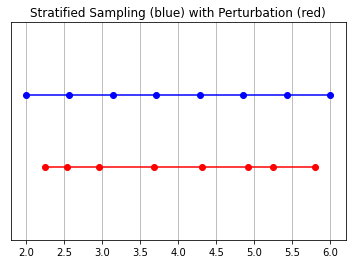
在这个模型中,相机最终拾取的 RGB 值是光样本沿着穿过该像素的光线的累积。 经典的体绘制方法是沿着这条射线累积然后积分点,在每个点估计射线在没有撞击任何粒子的情况下传播的概率。 因此,每个像素都需要沿穿过它的光线进行点采样。 为了最好地近似积分,他们的分层抽样方法是将空间均匀地划分为 N 个箱子,并从每个箱子中均匀地抽取样本。 分层采样方法不是简单地以规则间距绘制样本,而是允许模型对连续空间进行采样,从而调节网络以在连续空间上学习
def sample_stratified(
  rays_o: torch.Tensor,
  rays_d: torch.Tensor,
  near: float,
  far: float,
  n_samples: int,
  perturb: Optional[bool] = True,
  inverse_depth: bool = False
) -> Tuple[torch.Tensor, torch.Tensor]:
  r"""
  Sample along ray from regularly-spaced bins.
  """

  # Grab samples for space integration along ray
  t_vals = torch.linspace(0., 1., n_samples, device=rays_o.device)
  if not inverse_depth:
    # Sample linearly between `near` and `far`
    z_vals = near * (1.-t_vals) + far * (t_vals)
  else:
    # Sample linearly in inverse depth (disparity)
    z_vals = 1./(1./near * (1.-t_vals) + 1./far * (t_vals))

  # Draw uniform samples from bins along ray
  if perturb:
    mids = .5 * (z_vals[1:] + z_vals[:-1])
    upper = torch.concat([mids, z_vals[-1:]], dim=-1)
    lower = torch.concat([z_vals[:1], mids], dim=-1)
    t_rand = torch.rand([n_samples], device=z_vals.device)
    z_vals = lower + (upper - lower) * t_rand
  z_vals = z_vals.expand(list(rays_o.shape[:-1]) + [n_samples])

  # Apply scale from `rays_d` and offset from `rays_o` to samples
  # pts: (width, height, n_samples, 3)
  pts = rays_o[..., None, :] + rays_d[..., None, :] * z_vals[..., :, None]
  return pts, z_vals
7、层级体积抽样
早些时候当我说辐射场由多层感知器表示时,我可能有点撒谎。 事实上,它由两个多层感知器表示! 一个在粗略级别上操作,对场景的广泛结构属性进行编码。 另一个在精细的层次上细化细节,从而实现像网格和分支这样的薄而复杂的结构。 此外,它们接收到的样本是不同的,粗略模型在整个射线中处理广泛的、大部分规则间隔的样本,而精细模型则在具有显着信息的先验性强的区域进行磨练。
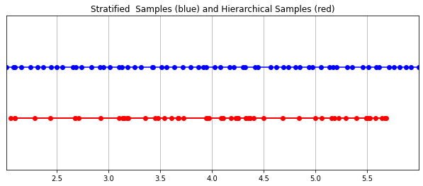
这种“磨练”过程是通过他们的分层体积抽样程序完成的。 3D 空间实际上非常稀疏且存在遮挡,因此大多数点对渲染图像的贡献不大。 因此,对很有可能对积分有贡献的区域进行过采样更为有益。 他们将学习到的归一化权重应用于第一组样本,以创建跨射线的 PDF。 然后,他们对该 PDF 应用逆变换采样以收集第二组样本。 该集合与第一集合组合并馈送到精细网络以产生最终输出。
def sample_hierarchical(
  rays_o: torch.Tensor,
  rays_d: torch.Tensor,
  z_vals: torch.Tensor,
  weights: torch.Tensor,
  n_samples: int,
  perturb: bool = False
) -> Tuple[torch.Tensor, torch.Tensor, torch.Tensor]:
  r"""
  Apply hierarchical sampling to the rays.
  """

  # Draw samples from PDF using z_vals as bins and weights as probabilities.
  z_vals_mid = .5 * (z_vals[..., 1:] + z_vals[..., :-1])
  new_z_samples = sample_pdf(z_vals_mid, weights[..., 1:-1], n_samples,
                          perturb=perturb)
  new_z_samples = new_z_samples.detach()

  # Resample points from ray based on PDF.
  z_vals_combined, _ = torch.sort(torch.cat([z_vals, new_z_samples], dim=-1), dim=-1)
  pts = rays_o[..., None, :] + rays_d[..., None, :] * z_vals_combined[..., :, None]  # [N_rays, N_samples + n_samples, 3]
  return pts, z_vals_combined, new_z_samples


def sample_pdf(
  bins: torch.Tensor,
  weights: torch.Tensor,
  n_samples: int,
  perturb: bool = False
) -> torch.Tensor:
  r"""
  Apply inverse transform sampling to a weighted set of points.
  """

  # Normalize weights to get PDF.
  pdf = (weights + 1e-5) / torch.sum(weights + 1e-5, -1, keepdims=True) # [n_rays, weights.shape[-1]]

  # Convert PDF to CDF.
  cdf = torch.cumsum(pdf, dim=-1) # [n_rays, weights.shape[-1]]
  cdf = torch.concat([torch.zeros_like(cdf[..., :1]), cdf], dim=-1) # [n_rays, weights.shape[-1] + 1]

  # Take sample positions to grab from CDF. Linear when perturb == 0.
  if not perturb:
    u = torch.linspace(0., 1., n_samples, device=cdf.device)
    u = u.expand(list(cdf.shape[:-1]) + [n_samples]) # [n_rays, n_samples]
  else:
    u = torch.rand(list(cdf.shape[:-1]) + [n_samples], device=cdf.device) # [n_rays, n_samples]

  # Find indices along CDF where values in u would be placed.
  u = u.contiguous() # Returns contiguous tensor with same values.
  inds = torch.searchsorted(cdf, u, right=True) # [n_rays, n_samples]

  # Clamp indices that are out of bounds.
  below = torch.clamp(inds - 1, min=0)
  above = torch.clamp(inds, max=cdf.shape[-1] - 1)
  inds_g = torch.stack([below, above], dim=-1) # [n_rays, n_samples, 2]

  # Sample from cdf and the corresponding bin centers.
  matched_shape = list(inds_g.shape[:-1]) + [cdf.shape[-1]]
  cdf_g = torch.gather(cdf.unsqueeze(-2).expand(matched_shape), dim=-1,
                       index=inds_g)
  bins_g = torch.gather(bins.unsqueeze(-2).expand(matched_shape), dim=-1,
                        index=inds_g)

  # Convert samples to ray length.
  denom = (cdf_g[..., 1] - cdf_g[..., 0])
  denom = torch.where(denom < 1e-5, torch.ones_like(denom), denom)
  t = (u - cdf_g[..., 0]) / denom
  samples = bins_g[..., 0] + t * (bins_g[..., 1] - bins_g[..., 0])

  return samples # [n_rays, n_samples]
8、训练
从论文中训练 NeRF 的标准方法大部分是你所期望的,但有一些关键差异。推荐的每网络 8 层和每层 256 维的架构在训练期间会消耗大量内存。他们缓解这种情况的方法是将前向传递分成更小的部分,然后在这些块中累积梯度。注意与小批量的区别;梯度是在一个小批量的采样光线中累积的,这些光线可能是成块收集的。如果你没有论文中使用的 NVIDIA V100 GPU 或性能相当的东西,可能必须相应地调整块大小以避免 OOM 错误。 Colab 笔记本使用更小的架构和更适中的分块大小。
我个人发现 NeRF 由于局部最小值而难以训练,即使选择了许多默认值也是如此。一些有用的技术包括在早期训练迭代和早期重新启动期间进行中心裁剪。随意尝试不同的超参数和技术,以进一步提高训练收敛性。
9、结论
辐射场标志着机器学习从业者处理 3D 数据的方式发生了巨大变化。 NeRF 模型和更广泛的可微分渲染正在迅速弥合图像创建和体积场景创建之间的差距。虽然我们走过的组件可能看起来非常复杂地组合在一起,但受此“原始的”NeRF 启发的无数其他方法证明,基本概念(连续函数逼近器 + 可微分渲染器)是构建各种解决方案的坚实基础无限的情况。我鼓励你自己尝试一下。渲染愉快!
10、参考文献
[1] Ben Mildenhall、Pratul P. Srinivasan、Matthew Tancik、Jonathan T. Barron、Ravi Ramamoorthi、Ren Ng — NeRF:将场景表示为视图合成的神经辐射场 (2020),ECCV 2020
[2] Julian Chibane、Aayush Bansal、Verica Lazova、Gerard Pons-Moll — 立体辐射场 (SRF):新场景稀疏视图的学习视图合成 (2021),CVPR 2021
[3] Alex Yu、Vickie Ye、Matthew Tancik、Angjoo Kanazawa — pixelNeRF:来自一个或几个图像的神经辐射场 (2021),CVPR 2021
[4] Zhengqi Li, Simon Niklaus, Noah Snavely, Oliver Wang — Neural Scene Flow Fields for Space-Time View Synthesis of Dynamic Scenes (2021), CVPR 2021
[5] Albert Pumarola、Enric Corona、Gerard Pons-Moll、Francesc Moreno-Noguer — D-NeRF:动态场景的神经辐射场 (2021),CVPR 2021
[6] Michael Niemeyer,Andreas Geiger — GIRAFFE:将场景表示为组合生成神经特征场(2021),CVPR 2021
[7] Zhengfei Kuang、Kyle Olszewski、Menglei Chai、Zeng Huang、Panos Achlioptas、Sergey Tulyakov — NeROIC:从在线图像集合中捕获和渲染神经对象,计算研究库 2022
[8] Konstantinos Rematas, Andrew Liu, Pratul P. Srinivasan,
Jonathan T. Barron、Andrea Tagliasacchi、Tom Funkhouser、Vittorio Ferrari — Urban Radiance Fields (2022),CVPR 2022
[9] Matthew Tancik、Vincent Casser、Xinchen Yan、Sabeek Pradhan、Ben Mildenhall、Pratul P. Srinivasan、Jonathan T. Barron、Henrik Kretzschmar — Block-NeRF:可扩展大场景神经视图合成 (2022),arXiv 2022
[10] Alex Yu、Sara Fridovich-Keil、Matthew Tancik、Qinhong Chen、Benjamin Recht、Angjoo Kanazawa — Plenoxels:没有神经网络的辐射场 (2022),CVPR 2022(口头)
[11] Ashish Vaswani、Noam Shazeer、Niki Parmar、Jakob Uszkoreit、Llion Jones、Aidan N. Gomez、Lukasz Kaiser、Illia Polosukhin — Attention Is All You Need (2017),NeurIPS 2017
[12] Nasim Rahaman、Aristide Baratin、Devansh Arpit、Felix Draxler、Min Lin、Fred A. Hamprecht、Yoshua Bengio、Aaron Courville — 关于神经网络的谱偏差(2019 年),第 36 届国际机器学习会议论文集( PMLR) 2019
原文链接:It’s NeRF From Nothing: Build A Complete NeRF with PyTorch
BimAnt翻译整理,转载请标明出处


